Now that we’re knee-deep into October, leaves are falling, temperatures are cooling, PSLs are flowing from Starbucks like water, and Halloween candy has completely taken over seasonal aisles in grocery stores across the country, it’s time for you to decide what candy to buy for trick-or-treaters.
Sure, you could take an economic approach and just get whatever’s cheapest (if you’re a grad student, I fully support this route), or you could just as well take an approach to give the people what they want!
The Data
To help you accomplish this, you all must know David Ng has provided us all with a wealth of critical data. Candy hierarchy data are available from the last four years. These survey data rank lots of different Halloween goodies by preference. Survey respondents let us know which items bring them “JOY,” which cause them “DESPAIR,” and which are just “MEH.” Results from the 2017 survey are here in this awesome graphic.
It’s important you become aware of these data now before you go out and purchase the goodies you’ll hand out this year. In this analysis, we’ll look at candy preference trends over time , so that you can be extra confident in your Halloween Candy purchase. It’s up to you whether you want to be a Halloween hero or the biggest dud on your block.
Thanks to Jenny Bryan for making me aware of these data with her tweet!
So you think you can (data) wrangle? Take a crack at this Halloween candy preference data! Looks like fun and a worthy challenge. https://t.co/d1TRvzXZL0
— Jenny Bryan (@JennyBryan) October 25, 2017
Time to Wrangle
First, we’ll just load the packages we’ll use throughout.
## load packages
library(janitor)
library(readr)
library(stringr)
library(reshape2)
library(readxl)
library(ggplot2)
library(dplyr)
There are a few quirks in these data. CSVs aren’t available for every year. Column names differ slightly. The 2014 and 2015 surveys didn’t have a “MEH” option. And, the raw data aren’t available for 2014 (just the summarized data). Thus, I decided to make all the data look like the 2014 data, calculating net feelies in each dataset from the raw data.
Note: If you saw me present this at R-Ladies Baltimore Launch and heard me say that I’d clean up this code before posting it online, I straight lied to you. It’s still not pretty. Life happens.
2017
## create directory for data
if(!dir.exists('candy_data')){
  dir.create('candy_data')
}

## download data from the Internet
if(!file.exists('candy_data/candyhierarchy2017.csv')) {
  download.file(url = 'http://www.scq.ubc.ca/wp-content/uploads/2017/10/candyhierarchy2017.csv',
                destfile = 'candy_data/candyhierarchy2017.csv')
}

## read data into R
candy17 <- read_csv("candy_data/candyhierarchy2017.csv")
names(candy17) <- names(candy17) %>% str_replace_all("\\\\xd5", "")
candy17 <- as.data.frame(candy17)

## determine which columsn we're interested in
cols_to_summarize <- grep("Q6", colnames(candy17))

## let's clean up those columns
df <- candy17[,cols_to_summarize] %>% clean_names()
colnames(df) <- gsub("q6_","",colnames(df))

## function to summarize despair and joy
summary_function <- function(x){
  a <- tabyl(x) %>%
    melt(id="x") %>%
    select(value) %>%
    t()
  return(a)
}

## get the names of all the columns we'll have in our output object
## who knows why I did it this way ¯\_(ツ)_/¯
x <- df[,2]
nameit <- tabyl(x) %>%
  melt(id="x") %>%
  mutate(category = paste0(x,"_",variable)) %>%
  select(category)

## run function to summarize joy and despair
output17 <- as.data.frame(t(apply(df, 2, summary_function)))
colnames(output17) <- nameit$category

## calculate net feelies
feelies17 = as.data.frame(as.numeric(output17$JOY_n - output17$DESPAIR_n))
rownames(feelies17) <- rownames(output17)
Data Summary
In 2017, observations were recorded from 2460 individuals and for 103 different Halloween items.
2016
## download data from the Internet
if(!file.exists('candy_data/BOING-BOING-CANDY-HIERARCHY-2016-SURVEY-Responses.xlsx')) {
  download.file(url = 'https://www.scq.ubc.ca/wp-content/uploads/2016/10/BOING-BOING-CANDY-HIERARCHY-2016-SURVEY-Responses.xlsx',
                destfile = 'candy_data/BOING-BOING-CANDY-HIERARCHY-2016-SURVEY-Responses.xlsx')
}

## read data into R
candy16 <- read_excel("candy_data/BOING-BOING-CANDY-HIERARCHY-2016-SURVEY-Responses.xlsx")
candy16 <- as.data.frame(candy16)
candy16 <- candy16[, !apply(is.na(candy16), 2, all)]

## get the columns you're interested in
cols_to_summarize <- grep("^\\[", colnames(candy16))
df16 <- candy16[,cols_to_summarize] %>% clean_names()

## use that function from above to summarize joy and despair for each item
output16 <- as.data.frame(t(apply(df16, 2, summary_function)))
colnames(output16) <- nameit$category

## calculate net_feeles
feelies16 = as.data.frame(as.numeric(output16$JOY_n - output16$DESPAIR_n))
rownames(feelies16) <- rownames(output16)
Data Summary
In 2016, observations were recorded from 1259 individuals and for 100 different Halloween items.
2015
## download data from the Internet
if(!file.exists('candy_data/CANDY-HIERARCHY-2015-SURVEY-Responses.xlsx')) {
    download.file(url = 'https://www.scq.ubc.ca/wp-content/uploads/2015/10/CANDY-HIERARCHY-2015-SURVEY-Responses.xlsx',
                destfile = 'candy_data/CANDY-HIERARCHY-2015-SURVEY-Responses.xlsx')
}

## read data into R
candy15 <- read_excel("candy_data/CANDY-HIERARCHY-2015-SURVEY-Responses.xlsx")

## get the columns you're interested in
cols_to_summarize <- grep("^\\[", colnames(candy15))
df15 <- as.data.frame(candy15[,cols_to_summarize])%>% clean_names()
colnames(df15)<-gsub("x_","",colnames(df15))

## see note in section above
x <- df15[,2]
nameit <- tabyl(x) %>%
  melt(id="x") %>%
  mutate(category = paste0(x,"_",variable)) %>%
  select(category)

## use that function from above to summarize joy and despair for each item
output15 <- as.data.frame(t(apply(df15, 2, summary_function)))
colnames(output15) <- nameit$category

## calculate net feelies
feelies15 = as.data.frame(as.numeric(output15$JOY_n - output15$DESPAIR_n))
rownames(feelies15) <- rownames(output15)
Data Summary
In 2015, observations were recorded from 5630 individuals and for 95 different Halloween items.
2014
## download data from the Internet
if(!file.exists('candy_data/CANDYDATA.xlsx')) {
    download.file(url = 'http://www.scq.ubc.ca/wp-content/uploads/2014/10/CANDYDATA.xlsx',
              destfile = 'candy_data/CANDYDATA.xlsx')
}

## read data into R & clean it up a little
candy14 <- read_excel("candy_data/CANDYDATA.xlsx") %>% clean_names %>%
  as.data.frame %>%
  filter(!is.na(item))
rownames(candy14) <- candy14$item
candy14 <- as.data.frame(t(candy14))
candy14<-clean_names(candy14)
colnames(candy14)<-gsub("x100","100",colnames(candy14))

candy14 <- as.data.frame(t(candy14))

## net feelies have already been calculated
feelies14 <- as.data.frame(as.numeric(as.character(candy14$net_feelies)))
rownames(feelies14) <- rownames(candy14)
Data Summary
In 2014, observations were recorded from 1286 individuals and for 86 different Halloween items.
Merging & Scaling
To complete this analysis, all four years of “feelies” data are combined into a single data frame. They are then scaled within each year so that the most favorable candy (brings the most relative “JOY”) receives a score of +1 while the least favorable (brings the most relative “DESPAIR”) receives a score of -1.
## merge all these data together
combined_all <- merge(feelies14,feelies15,by = "row.names", all = TRUE) %>%
  merge(.,feelies16,by.x = "Row.names",by.y = "row.names", all = TRUE) %>%
  merge(.,feelies17,by.x = "Row.names",by.y = "row.names", all=TRUE)
combined_all <- as.data.frame(combined_all)
colnames(combined_all) <- c("row.names","x2014","x2015","x2016","x2017")

## scale all values between -1 and 1 within a year
scalefunc <- function(x){
  minx = min(x, na.rm = TRUE)
  maxx = max(x, na.rm = TRUE)
  val= 2*((x - minx)/(maxx - minx))-1
  return(val)
}
out_all <- as.data.frame(apply(combined_all[,2:5],2,scalefunc))
out_all$row.names <- as.character(combined_all$row.names)

## calculate a few things we may use to order the graph
## calculate sum, normalized by number of years question was asked
out_all$sum <- rowSums(out_all[,1:4],na.rm=TRUE)
isNA <- function(x){sum(is.na(x))}
out_all$isNA <- apply(out_all,1,isNA)
out_all$sum_NA <- out_all$sum/(4-out_all$isNA)
out_all <- out_all %>% arrange(sum_NA)
Give the People What They Want!
What you’ve been waiting for - the results! Each year is a different color point on the graph (see legend on the plot). Rows are ordered such that items with the most positive net feelies are listed at the top of the graphic (Halloween Hero territory!) and those that consistently cause the most despair (Neighborhood Dud Land) are at the bottom.
## tidy data format!
data_all <- melt(out_all, id.vars='row.names',
                 variable.name='Year', value.name = "net_feelies") %>%
  mutate(item_name = gsub("_", " ",row.names))

## let's plot!
data_all %>%
  filter(Year=="x2014" | Year=="x2015" | Year=="x2016" | Year=="x2017") %>%
  ggplot(., aes(x = factor(item_name, level = unique(item_name)),
                y = net_feelies,
                color = Year)) +
  geom_point(size = 4) +
  scale_colour_manual(
    labels = c("x2014" = "2014",
               "x2015" = "2015",
               "x2016" = "2016",
               "x2017" = "2017"),
    values = c("x2014" = "#FFEE4A",
               "x2015" = "#FE9600",
               "x2016" = "gray48",
               "x2017" = "#77477E")) +
  geom_segment(aes(x = item_name,
                   xend = item_name,
                   y = -1,
                   yend = 1),
               linetype = "dashed",
               size = 0.1) +   # Draw dashed lines
  scale_x_discrete(labels = function(y) str_wrap(y, width = 47)) +
  labs(title ="Candy Preferences Over Time",
       subtitle ="So Much Candy Survey",
       caption ="source: http://www.scq.ubc.ca/so-much-candy-data-seriously/",
       x="",
       y="net feelies (scaled)") +
  coord_flip() +
  theme(legend.position = c(-0.7, 0.9),
        legend.text = element_text(size = 16),
        axis.text.x = element_text(size = 16, hjust = 0.5),
        axis.text.y = element_text(size = 11),
        axis.title.y = element_text(size = 14),
        legend.title = element_text(size = 20),
        plot.title = element_text(size = 24, hjust = 1.2, color = "#77477E"),
        plot.subtitle = element_text(size = 16, hjust = -0.45, color = "#FE9600"))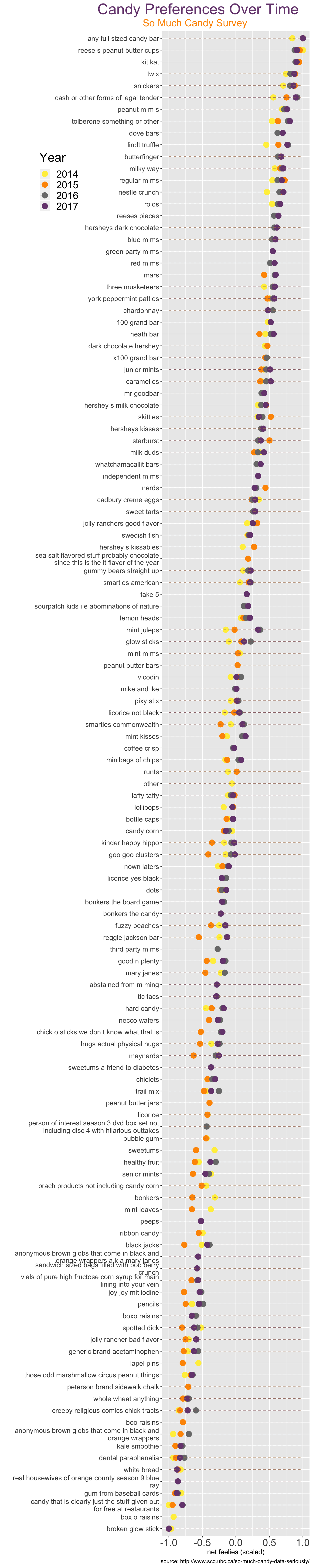
Take-Away Messages
When I look at this plot, I conclude that candy preferences do not vary wildly from year to year. That’s good for you! What the people have liked in the past is likely to be what they’ll like this year!
For items in the middle of the plot where scaled net feelies appear to differ more from year to year, I want to remind you that “MEH” was not an option in 2014 and 2015, suggesting that when not given the “MEH” choice, people tend to say “DESPAIR.”
Halloween Hero Territory
Probably unsurprisingly, full-sized candy bars are the bee’s knees on Halloween. But, we’re not all made of money. Fortunately, Reese’s peanut butter cups, Kit Kat bars, Twix, and Snickers consistently bring almost as much joy as full-sized candy bars. So, if you want to maximize the joy your treats bring your trick-or-treaters while not breaking the bank, opt for one of these classics!
Neighborhood Dud Land
On the other end, if you want to be known as the neighborhood’s worst stop for Halloween treats, give out broken glow sticks! Similarly, raisins, dental paraphernalia, and sidewalk chalk are also likely to land you on the worst-candy neighborhood list.
The Sleepers
If you’re driven to be unique, Dove bars, Lindt truffles, and Mars are less popular (as determined by my many years of trick-or-treating experience) but bring joy the masses (as proven by these data)!
Personal Hot-Take
Personally, I think Kit Kats are way too high on this list and are a completely mediocre (at best) candy.
Similarly, I take offense to the fact that the respondents’ preferences are so heavily skewed to chocolate candy. Don’t get me wrong, chocolate is great. But that said, the first non-chocolate item to show up is chardonnay. Chardonnay!?!?! While delicious, is certainly not a Halloween candy to be given out to minors. I’m here to lobby for the joy brought to me by gummy candy! Swedish fish! Sour Patch Kids! Good N Plenty! These candies are getting the damn shaft on this list.
Finally, if you ever find yourself with a kale smooothie on your hands that you’re not interested in drinking, I’d be happy to take it off your hands.
** Edit 11/10/18: Thanks to Leo Collado-Torres for helpfully pointing out that wget won’t work on a PC and suggesting I use download.file() instead.