Background
I previously wrote Part I in this short series describing my first course here at UCSD, specifically focusing on three things than went well…and three that went er not so well. Now, as I sit in the time period after having submitted final grades but before having access to student evaluations, I wanted to take a few minutes to draft a few posts using the data I collected from students throughout the course to tell a short story about what they, en masse, thought of the course.
The Data
For privacy reasons, none of the data I use are going to be identifiable or individual-level, but I wanted to at least share the sources of the data I collected from the 326 students in the course:
- Roster information - includes their official major (N=326)
- Pre-course survey - asked about demographic, educational background & interests, and course topic familiarity. I also asked a few random questions, mostly to be used to demonstrate different types of distributions/variable types (i.e. “Do you have a pet?”, “What’s your favorite color”) (N=277)
- Daily iclicker responses - individual responses recorded for each lecture; opportunity for extra credit if students attended >=75% of classes (mean attendance: 211, range:121-299)
- Exam, Reading Quizzes, & Assignment Scores - There were two exams, 5 reading quizzes, 4 assignments, and 1 final project.
- Mid-course Survey - mostly asked how this course ranked relative to their other courses and asked for positive and negative feedback about COGS9 (N=159)
- Post-course Survey - asked about course topic familiarity (N=151)
Aside from grades, you’ll note that I don’t have data from everyone across every piece of information collected. Such is life in data collection in the classroom.
# how much material presented has been new to you
new_material <- read_csv("cogs9_data/material_new.csv")
new_material_respondedall <- read_csv("cogs9_data/material_new_subset.csv")
# pre-post for topic familiarity
topics <- read_csv("cogs9_data/pre_post_survey.csv")
# lecture attendance
lecture <- read_csv("cogs9_data/attendance.csv")
The Questions
There are tons of questions that can be asked of these data, but I’m just going to focus on three for this post:
- Are students learning new information?
- Do students have an improved understanding of course topics?
- Does attending lecture matter?
Are Students Learning?
To answer this question, I asked the same question at three points throughout the course via iclicker. For the topics covered in the beginning, middle, and final third of the courses students were reminded of the topics covered and then asked “What percentage of the course material has been new to you?” Students were able to select quintiles including percentages ranging from 0-100%.
The reason I did this is simply because this is an introductory course with students from varied backgrounds and I didn’t really know what to expect, nor did I have any idea of whether or not this would change over the course of the quarter.
While this is self-reported, that’s really what I was interested in. Have students seen this information before or are they learning new stuff?
Proportion of new material
ggplot(new_material, aes(value, freq*100)) +
  geom_bar(stat = "identity") +
  facet_wrap(~key) +
  theme_bw(base_size=10) +
  labs(y = "proportion of responses",
       x = "What proportion of material is new to you?",
       title = "Students are largely getting exposed to some new information",
       subtitle = "But, for most students, some amount of material has been covered elsewhere previously" ) +
  theme(panel.grid = element_blank())
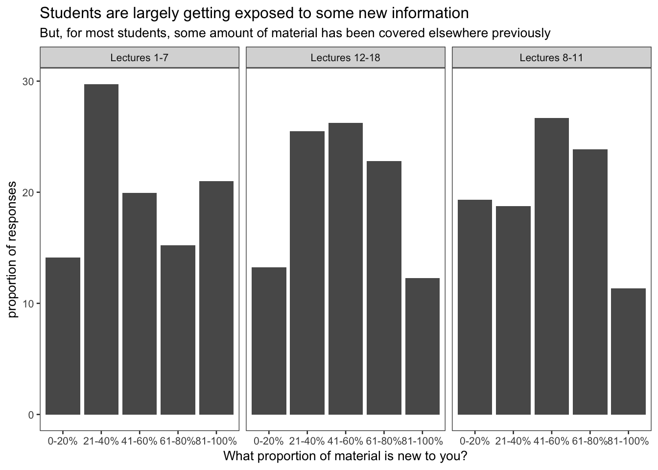
This first panel shows that overall during the first third of the class (ethics, data, and data wrangling), most people learned something new in the material covered, but a lot of people had seen a fair amount of the material before. This felt right for an intro class, but I don’t really have much to compare it with. For the second third (data visualization, descriptive and exploratory data analysis), most people were somewhere in the middle - it wasn’t all new but they had seen a fair amount of it before. The final third (inference, machine learning, geospatial analysis, and text analysis) had most people having been exposed to some material before, with fewer having the vast majority of the material be new.
Shift in proportion over course
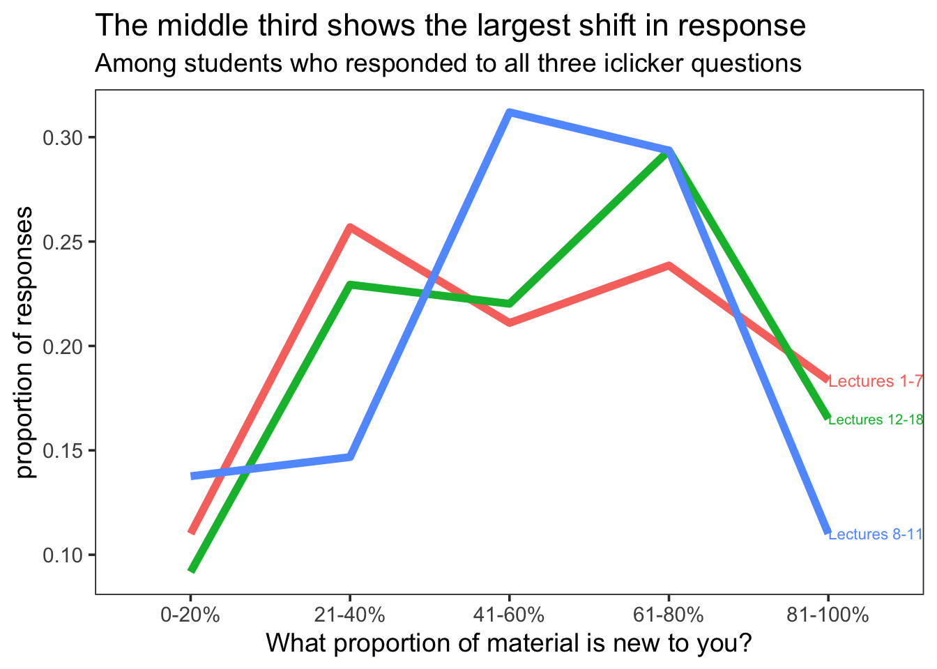
In the previous plot I included all responses; however, I was curious to see if the proportion changed over time among students who responded to all three inquiries. Below only responses from students who responded all three times are summarized.
p <- ggplot(data = new_material_respondedall, aes(x = value, y = freq, group = key)) +
  geom_line(aes(color = key), size = 2) +
  theme_bw(base_size=14) +
  labs(y="proportion of responses",
       x="What proportion of material is new to you?",
       title = 'The middle third shows the largest shift in response',
       subtitle = "Among students who responded to all three iclicker questions" ) +
  theme(panel.grid = element_blank())
direct.label(p,"last.qp")
We see that the proportion of responses shows the largest shift in the 41-60% bin for the middle third of the course (data visualization and EDA focused lectures). The first and last third of the course have a fairly consistent pattern. I did look to see if individual responses stayed consistent, and while I’m not showing the data here because that starts to get at individual level data, what I’ll say is that there were all types of people. Some who responded consistently that the same proportion of material is new and many who changed responses over the course of the quarter. What was not seen frequently (as one may expect) were shifts from one extreme to the other. Very few people went from 0-20% of the material being new in one third of the course to 81-100% of the material being new in another third of the course. (Also, I don’t love this visualization so if someone has a suggestion for how to display this information better, let me know- I’d love to hear suggestions.)
Improved understanding of course topics?
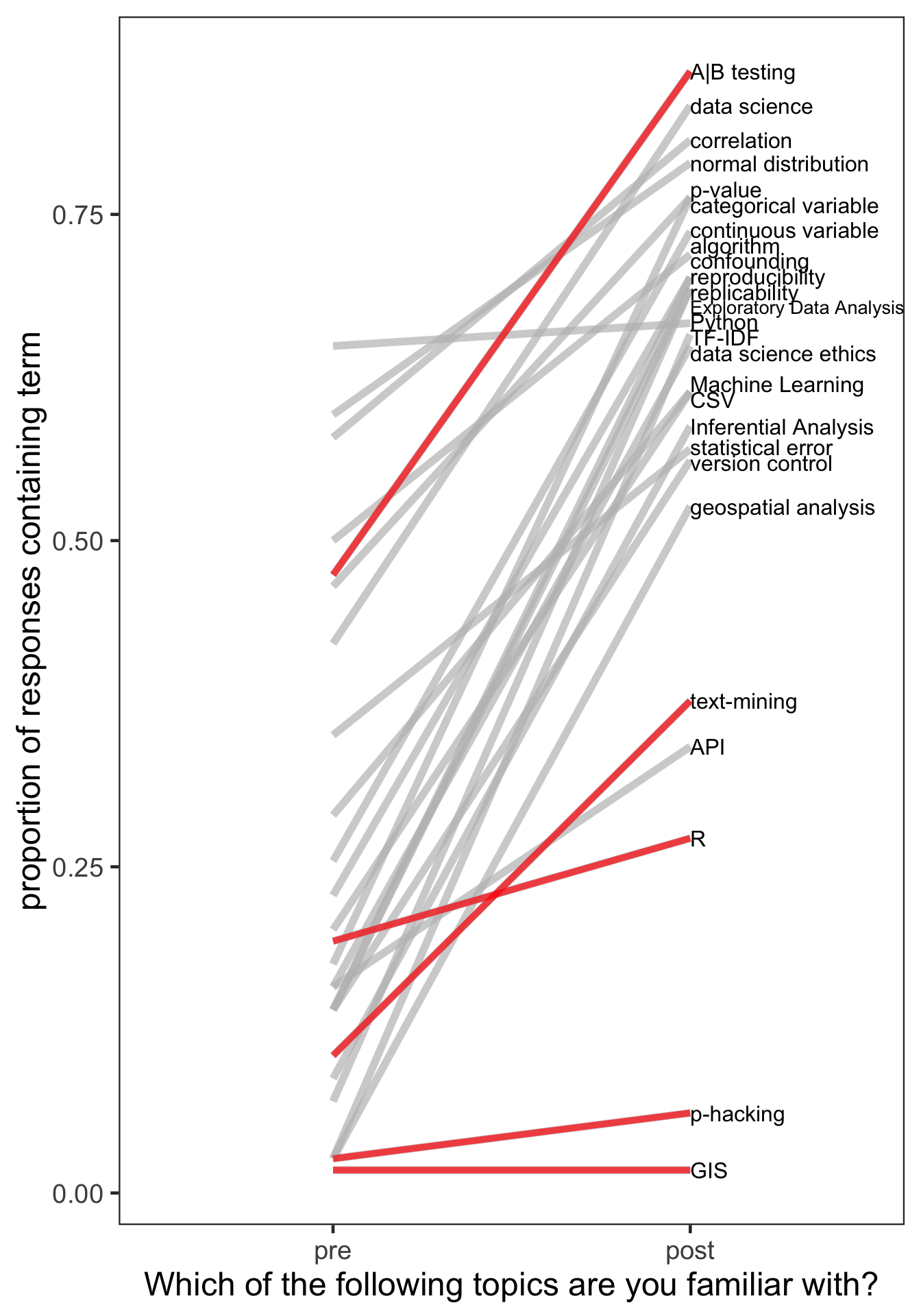
If students are learning new material, what are they learning. I asked students in the pre- and post- course surveys to answer the following: “Which of the following topics are you familiar with? (Here, familiar means you could explain the topic clearly to a friend without Googling it first.) Check all that apply.” Most topics were topics we would cover in the course, but I threw in a few controls - topics that are related to data science but that we weren’t going to cover in this course. Those “controls” are highlighted in red below.
not <- c("R", "A|B testing", "p-hacking", "text-mining", "GIS")
d <- topics %>%
  mutate(time = fct_relevel(topics$time, "pre"),
         notcovered = ifelse(key %in% not, TRUE, FALSE))
d_filtered <- d %>% filter(notcovered)

ggplot() +
  geom_line(data=d, aes(x=time,y=value, group = key, color=key), size = 2, color = alpha("grey", 0.7)) +
  guides(color=FALSE) +
  geom_dl(data=d, aes(x=time,y=value, label=key),  method="last.qp") +
  geom_line(data= d_filtered, aes(x = time, y = value, group = key), size = 1.7, color = alpha("red", 0.7)) +
  theme_bw(base_size=18) +
  # scale_x_discrete(expand = c(0, .1)) +
  labs(y="proportion of responses containing term", x="Which of the following topics are you familiar with?") +
theme(panel.grid = element_blank()) 
Overall, students felt more familiar with topics covered at the end of the course, which is great to see (at a bare minimum). I’ll note that while A|B testing was planned to be covered in COGS9, an example of A|B testing was explained by one of our guest speakers. We then reviewed the following lecture what our guest lecturer spoke about. So, students were exposed to A|B testing, and I kind of love that students feel they have a grasp on it now!
As for text mining and R, we didn’t cover those in detail, although the discussion of what R is relative to Python and data science was touched on. I didn’t mention the words “p-hacking” or “GIS” at all in the course…although, I probably should cover p-hacking in the future.
The final two topics I want to mention are “Python”…a rather flat line, and “API”, a line showing that most people don’t have an understanding despite it having been covered. For Python, we used Python in the course but only minimally to wrangle a dataset and create basic visualizations. If you already know Python, this is pretty simple. And, if you didn’t, you could totally pass the class without mastering this. So, the fact that this didn’t change over the course of the quarter is pretty understandable. It also demonstrates that COGS9 is a weird course where more than half of students program and the other half do not. As for API, this may have been the topic I did the worst job explaining during lecture. It felt bad after the lecture. And, their exams demonstrated that they didn’t get it. So, this line makes sense to me. Something to improve for the future!
Does attending lecture matter?
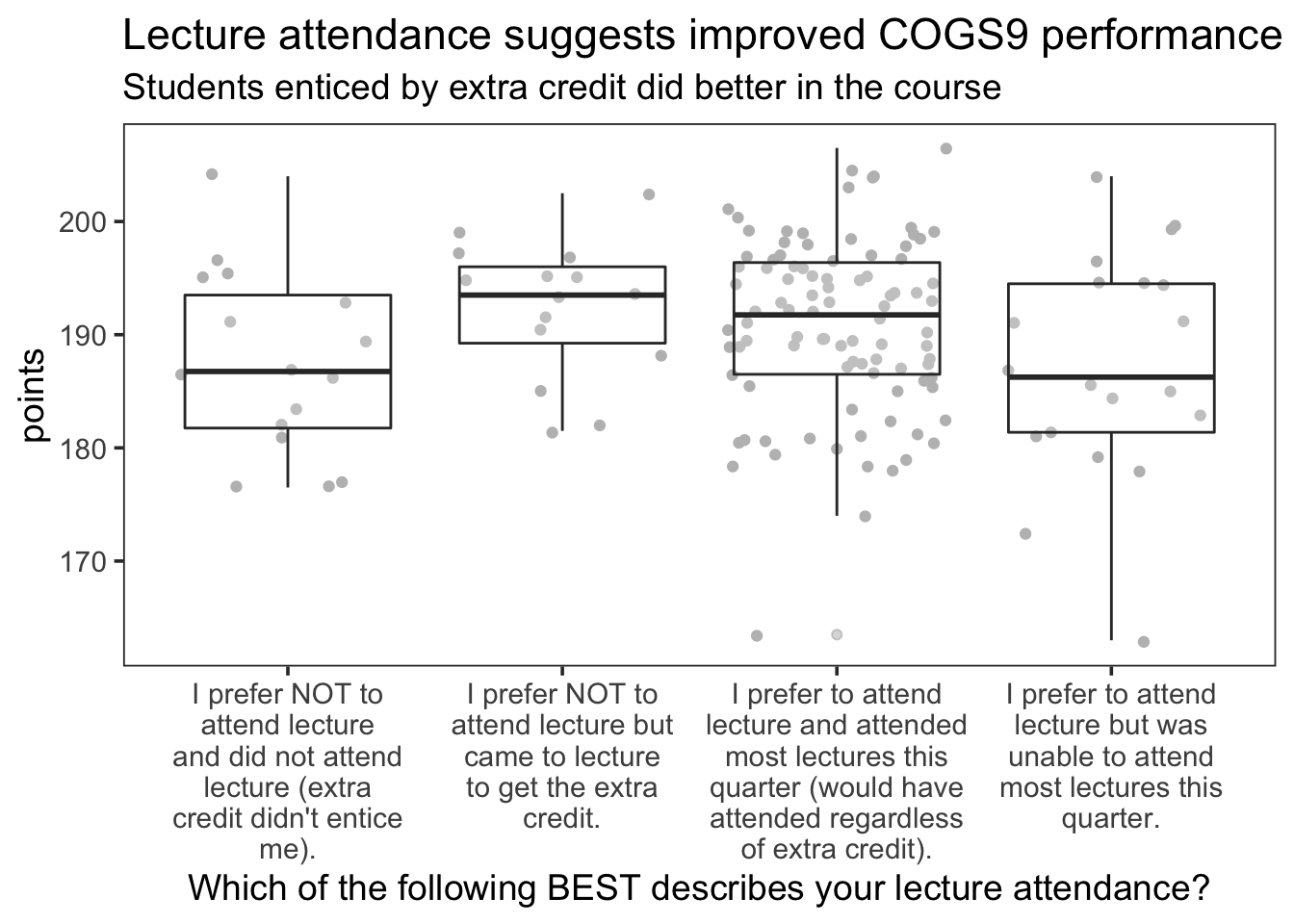
I have an attendance policy where students are not penalized for skipping lecture, but I offer extra credit if students attend at least 75% of the lectures (measured by iclicker response). I was really curious to see if students who attend lecture tend to do better in the course. Further, I was most interested in those students who don’t like to come to lecture but came for the extra credit. Below I’ve plotted the number of points students received (without the extra credit) broken down by their self reported feelings toward lecture attendance. Data are included for the 148 students who responded to the attendance question on the post-course survey.
ggplot(lecture, aes(x=lecture_attendance, total_points)) +
  geom_jitter(color="gray") +
  geom_boxplot(alpha=0.2) +
  scale_x_discrete(labels = function(x) str_wrap(x, width = 20)) +
  theme_bw(base_size=14) +
  labs(y = "points",
       x = "Which of the following BEST describes your lecture attendance?",
       title = "Lecture attendance suggests improved COGS9 performance",
       subtitle = "Students enticed by extra credit did better in the course") +
  theme(panel.grid = element_blank())
Here, we do see that those who attended lecture do better in the course overall. This convinces me to keep this attendance policy for the coming quarter.